Logic Gates

---

Let's load some libraries we will need.

import numpy as np
import scipy.integrate
import scipy.optimize

import matplotlib.pyplot as plt
%matplotlib inline

figsize=(6, 4.5)


# drawing digital circuits:
# %pip install schemdraw
import schemdraw
import schemdraw.logic as logic
import schemdraw.elements as elm

The Inverter

Let us quickly recall the inverter (INV gate) that negates an input X resulting in an output Z = INV(X).

with schemdraw.Drawing() as d:
    inv = d.add(logic.Not().label('INV', loc='bottom'))
    d.add(elm.Label().at((inv.in1[0]-1.5, inv.in1[1])).label('X', halign='right'))
    d.add(elm.Label().at((inv.out[0]+1.5, inv.out[1])).label('Z', halign='left'))

We will use the Python library dnaplotlib for plotting circuits. The library uses the SBOL standard for symbols. You can find an overview on the supported symbols at their visual glyphs page.

# %pip install dnaplotlib
import dnaplotlib as dpl

# Create DNA renderer
dr = dpl.DNARenderer()
renderers = dr.SBOL_part_renderers()

# --- Define design ---
# --- A gate ---
p0 = {
        'type': 'Promoter',
        'fwd': True,
        'opts': {
            'label':'PX',
            'label_size':10,
            'label_y_offset': -5,
            'color':[0.8, 0.8, 0.8],
        },
    }
rbs0 = {
        'type': 'RBS',
        'fwd': True,
        'opts': {
            'color':[0.8, 0.8, 0.8],
        }
    }
cds0 = {
        'type': 'CDS',
        'fwd': True,
        'opts': {
            'color':[0.38, 0.82, 0.32],
            'label':'X',
            'label_size':10
        },
    }
t0 = {
        'type': 'Terminator',
        'fwd': True,
    }

# --- inverter gate ---
p2 = {
        'type': 'Promoter',
        'fwd': True,
        'opts': {
            'color': [0.38, 0.82, 0.32],
            'label': 'PZ',
            'label_size':10,
            'label_y_offset': -5
        },
    }
rbs2 = {
        'type': 'RBS',
        'fwd': True,
    }
cds2 = {
        'type': 'CDS',
        'fwd': True,
        'opts': {
            'label':'Z',
            'label_size':10
        },
    }
t2 = {
        'type': 'Terminator',
        'fwd': True,
    }

# --- Define regulation ---
regulations = [
    {
        'from_part': cds0,
        'to_part': p2,
        'type': 'Repression',
        'opts': {
            'color': [0.38, 0.82, 0.32],
        }
    }
]

design = [
    p0, rbs0, cds0, t0,
    p2, rbs2, cds2, t2,
]

# --- Render DNA ---
fig, ax = plt.subplots(figsize=(6, 4))

# orange gate box
gate_x = [71, 71, 150, 150]
gate_y = [25, -20, -20, 25]
ax.fill(gate_x, gate_y, color='orange', alpha=0.3)

start_pos, end_pos = dr.renderDNA(
    ax=ax,
    parts=design,
    regs=regulations,
    part_renderers=renderers,
    reg_renderers= dr.std_reg_renderers(),
)

ax.annotate(
    'in: X',
    xy=(60, 25),
    xytext=(60, 25),
    fontsize=10,
    ha='center',
    va='center'
)
ax.annotate(
    'out: Z rate',
    xy=(110, -15),
    xytext=(130, -15),
    arrowprops=dict(arrowstyle="<-", color='black', lw=1.5),
    fontsize=10,
    ha='center',
    va='center'
)

ax.set_xlim(start_pos - 1, end_pos + 1)
ax.set_ylim(-40, 40)
ax.set_axis_off()
plt.tight_layout()

Conceptually, here, the gate starts after CDS X, with the concentration X being the input, and ends with CDS Z, with the production rate of Z being the output. We mark the components that belong to the gate in orange.

We had approximated the stead-state expression rate of the output gene $Z$ with a Hill function:

\begin{align} \beta(X) = \beta_{\max} \frac{1}{1+X/K_\mathrm{d}} \end{align}

where $\beta_{\max}$ is the maximal production rate and $K_d$ the dissociation constant $k_-/k_+$. Generalizing this to higher order Hill coefficients $n \geq 1$ we can write \begin{align} \beta(X) = \beta_{\max} \frac{1}{1+(X/K_\mathrm{d})^n} \end{align} The result is a sharper, say "more digital", dependency of the production rate with respect to the repressor $X$.

Side note: While we derived the approximation for $n=1$ for activation and repression in previous lectures, the case $n > 1$ is only phenomenologically, here. One can, however, derive the case for larger $n$ as an approximation of certain types of activation and repression, e.g., with so-called cooperativity.

We are further including some leaky production rate that we will specify via a minimal and maximal production rate

\begin{align} \beta(X) = \beta_{\min} + \frac{\beta_{\max} - \beta_{\min}}{1+(X/K_\mathrm{d})^n} \end{align}

One readily verifies that the inverter is consistent with the operational corners: $\beta(0) = \beta_{\max}$ (= logical 1) and $\lim_{X \to \infty} \beta(X) = \beta_{\min}$ (= logical 0).

Further, observe that the input domain (concentrations or counts) is $[0, \infty)$ and the output domain (rates) is $[\beta_{\min},\beta_{\max}]$. This is not to be confused with classical digital circuits where we could expect all signals to be in a normalized $[0,1]$.

Let us visualize the steady-state of the output vs. the input. One calls this the transfer characteristics or transfer function of the gate.

def inv(x: np.ndarray, Kd : float = 1.0, n : float = 1.0, beta_min : float = 1.0, beta_max : float = 5.0) -> np.ndarray:
    return beta_min + (beta_max - beta_min) / (1 + x / Kd)**n

x = np.linspace(0, 100, 10000)
plt.figure(figsize=(4,4))
ax = plt.gca()
plt.plot(x, inv(x, n= 1.0), 'blue', label='n = 1')
plt.plot(x, inv(x, n= 2.0), 'green', label='n = 2')
ax.set_ylim(1, 5)
plt.title("Transfer characteristics of INV")
plt.xlabel("X (concentration)")
plt.ylabel("Z (rate)")
plt.legend()

<matplotlib.legend.Legend at 0x118279e50>

There is not much visible in a linear plot, so let us visualize the transfer characteristics in a log-log plot to see the behavior for low as well as for high input concentrations.

x = np.linspace(0, 100, 10000)
plt.figure(figsize=(4,4))
ax = plt.gca()
plt.plot(x, inv(x, n= 1.0), 'blue', label='n = 1')
plt.plot(x, inv(x, n= 2.0), 'green', label='n = 2')
ax.set_yscale('log')
ax.set_xscale('log')
ax.set_ylim(0.9, 5.1)
ax.set_yticks(range(1,6),labels=range(1,6))
plt.title("Transfer characteristics of INV")
plt.xlabel("X (concentration)")
plt.ylabel("Z (rate)")
plt.legend()

<matplotlib.legend.Legend at 0x10ef4ec00>

Changing the Input and Output Signal

There is a problem though with this characterization of gates. How do we compose gates with the input being in terms of concentrations and the output in terms of an expression rate.

A solution is to "box" the gate differently. We can as well consider the inputs to be the promoter activity (a rate) of the PX promoter. The promoter PX itself is not part of the gate. For consistency, we can then also choose the promoter activity of PZ as the output signal. While the output promoter activity will probably be proportional to the expression rate of Z, the rates may be not identical (RNAPs may prematurely stop).

Promoter activity may be measured in several units. Examples are RNAP/s or relative measures like Relative Promoter Units (RPU).

Now we can nicely compose gates. Let's visualize the new understanding of an INV gate:

# --- Define design ---
# --- A gate ---
p0 = {
        'type': 'Promoter',
        'fwd': True,
        'opts': {
            'label':'PX',
            'label_size':10,
            'label_y_offset': -5,
            'color':[0.8, 0.8, 0.8],
        },
    }
rbs0 = {
        'type': 'RBS',
        'fwd': True,
    }
cds0 = {
        'type': 'CDS',
        'fwd': True,
        'opts': {
            'color':[0.38, 0.82, 0.32],
            'label_size':10
        },
    }
t0 = {
        'type': 'Terminator',
        'fwd': True,
    }

# --- inverter gate ---
p2 = {
        'type': 'Promoter',
        'fwd': True,
        'opts': {
            'color': [0.38, 0.82, 0.32],
            'label': 'PZ',
            'label_size':10,
            'label_y_offset': -5
        },
    }

# --- Define regulation ---
regulations = [
    {
        'from_part': cds0,
        'to_part': p2,
        'type': 'Repression',
        'opts': {
            'color': [0.38, 0.82, 0.32],
        }
    }
]

design = [
    p0, rbs0, cds0, t0,
    p2,
]

# --- Render DNA ---
fig, ax = plt.subplots(figsize=(6, 4))

# orange gate boxes
gate_x = [15, 15, 70, 70]
gate_y = [25, -20, -20, 25]
ax.fill(gate_x, gate_y, color='orange', alpha=0.3)

gate_x2 = [73, 73, 150, 150]
gate_y2 = [25, -20, -20, 25]
ax.fill(gate_x2, gate_y2, color='orange', alpha=0.3)

start_pos, end_pos = dr.renderDNA(
    ax=ax,
    parts=design,
    regs=regulations,
    part_renderers=renderers,
    reg_renderers= dr.std_reg_renderers(),
)

ax.annotate(
    'in: PX activity (rate)',
    xy=(1, -15),
    xytext=(31, -15),
    arrowprops=dict(arrowstyle="<-", color='black', lw=1.5),
    fontsize=10,
    ha='center',
    va='center'
)
ax.annotate(
    'out: PZ activity (rate)',
    xy=(74, -15),
    xytext=(104, -15),
    arrowprops=dict(arrowstyle="<-", color='black', lw=1.5),
    fontsize=10,
    ha='center',
    va='center'
)

ax.set_xlim(start_pos - 1, end_pos + 1)
ax.set_ylim(-40, 40)
ax.set_axis_off()
plt.title("Genetic design of an INV")
plt.tight_layout()

The gate has two constructs that can be placed on different positions on the DNA.

Like, before, a leaky Hill model turns out to be a good approximation for the transfer characteristics of the INV gate.

\begin{align} Z(X) = Z_{\min} + \frac{Z_{\max} - Z_{\min}}{1+(X/K_\mathrm{d})^n} \end{align}

Let us verify that the function correctly captures an INV.

X	expected Z	model Z
low $X$ = 0	1	$ Z(0) = Z_{\max} = $ 1
high $X$ = 1	0	$ \lim_{X \to \infty} Z(X) = Z_{\min} = $ 0

The NOR gate

Let us generalize the INV to a 2 input gate. Nothing prevents us from expressing X from two different input promoters. The resulting logic is the one of a NOR.

with schemdraw.Drawing() as d:
    nor = d.add(logic.Nor().label('NOR', loc='bottom'))
    d.add(elm.Label().at((nor.in1[0]-0.2, nor.in1[1])).label('X', halign='right'))
    d.add(elm.Label().at((nor.in2[0]-0.2, nor.in2[1])).label('Y', halign='right'))
    d.add(elm.Label().at((nor.out[0]+0.1, nor.out[1])).label('Z', halign='left'))

The genetic design of such a NOR looks like this:

# --- Define design ---
# --- A gate ---
p0 = {
        'type': 'Promoter',
        'fwd': True,
        'opts': {
            'label':'PX',
            'color':[0.8, 0.8, 0.8],
            'label_size':10,
            'label_y_offset': -5
        },
    }
rbs0 = {
        'type': 'RBS',
        'fwd': True,
        'opts': {
            'color':[0.8, 0.8, 0.8],
        }
    }
cds0 = {
        'type': 'CDS',
        'fwd': True,
        'opts': {
            'color':[0.38, 0.82, 0.32],
            'label_size':10
        },
    }
t0 = {
        'type': 'Terminator',
        'fwd': True,
    }

# --- B gate ---
p1 = {
        'type': 'Promoter',
        'fwd': True,
        'opts': {
            'label':'PY',
            'label_size':10,
            'label_y_offset': -5,
            'color':[0.8, 0.8, 0.8],
        },
    }
rbs1 = {
        'type': 'RBS',
        'fwd': True,
        'opts': {
            'color':[0.8, 0.8, 0.8],
        }
    }
cds1 = {
        'type': 'CDS',
        'fwd': True,
        'opts': {
            'color':[0.38, 0.82, 0.32],
            'label_size':10
        },
    }
t1 = {
        'type': 'Terminator',
        'fwd': True,
    }

# --- inverter gate ---
p2 = {
        'type': 'Promoter',
        'fwd': True,
        'opts': {
            'color': [0.38, 0.82, 0.32],
            'label': 'PZ',
            'label_size': 10,
            'label_y_offset': -5
        },
    }

# --- Define regulation ---
regulations = [
    {
        'from_part': cds0,
        'to_part': p2,
        'type': 'Repression',
        'opts': {
            'color': [0.38, 0.82, 0.32],
        }
    },
    {
        'from_part': cds1,
        'to_part': p2,
        'type': 'Repression',
        'opts': {
            'color': [0.38, 0.82, 0.32],
        }
    }
]

design = [
    p0, rbs0, cds0, t0,
    p1, rbs1, cds1, t1,
    p2,
]

# --- Render DNA ---
fig, ax = plt.subplots(figsize=(6, 3))

# orange gate boxes
gate_x = [13, 13, 70, 70]
gate_y = [30, -20, -20, 30]
ax.fill(gate_x, gate_y, color='orange', alpha=0.3)

gate_x2 = [85, 85, 142, 142]
gate_y2 = [30, -20, -20, 30]
ax.fill(gate_x2, gate_y2, color='orange', alpha=0.3)

gate_x3 = [145, 145, 160, 160]
gate_y3 = [30, -20, -20, 30]
ax.fill(gate_x3, gate_y3, color='orange', alpha=0.3)

start_pos, end_pos = dr.renderDNA(
    ax=ax,
    parts=design,
    regs=regulations,
    part_renderers=renderers,
    reg_renderers= dr.std_reg_renderers(),
)

ax.annotate(
    'in X',
    xy=(0, -15),
    xytext=(15, -15),
    arrowprops=dict(arrowstyle="<-", color='black', lw=1.5),
    fontsize=10,
    ha='center',
    va='center'
)
ax.annotate(
    'in Y',
    xy=(75, -15),
    xytext=(90, -15),
    arrowprops=dict(arrowstyle="<-", color='black', lw=1.5),
    fontsize=10,
    ha='center',
    va='center'
)
ax.annotate(
    'out Z',
    xy=(145, -15),
    xytext=(160, -15),
    arrowprops=dict(arrowstyle="<-", color='black', lw=1.5),
    fontsize=10,
    ha='center',
    va='center'
)

ax.set_xlim(start_pos - 1, end_pos + 1)
ax.set_ylim(-40, 40)
ax.set_axis_off()
plt.title("Genetic design of a NOR (split gate)")
plt.tight_layout()

This design is called the Split Gate design, as opposed to another design that we will discuss in a second.

With the concentrations of the repressors adding up, a simple summation of input rates $X$ and $Y$ is a plausible assumption. In this case we obtain

\begin{align} Z(X, Y) &= Z_{\min} + \frac{Z_{\max} - Z_{\min}}{1+((X + Y)/K_\mathrm{d})^n} \end{align}

Let us verify that the function correctly captures a NOR.

X	Y	expected Z	model Z
low $X$ = 0	low $X$ = 0	1	$ Z(0,0) = Z_{\max} = $ 1
low $X$ = 0	high $X$ = 1	0	$ \lim_{Y \to \infty} Z(X,Y) = Z_{\min} = $ 0
high $X$ = 1	low $X$ = 0	0	$ \lim_{X \to \infty} Z(X,Y) = Z_{\min} = $ 0
high $X$ = 1	high $X$ = 1	0	$ \lim_{X,Y \to \infty} Z(X,Y) = Z_{\min} = $ 0

We can plot the steady-state of this function

def contour_fun(x: np.ndarray, y: np.ndarray, z: np.ndarray, title: str | None=None):
    """
    Make a filled contour plot given x, y, z
    in 2D arrays.
    """
    plt.figure()
    CS = plt.contourf(x, y, z)
    plt.colorbar(CS)
    if title is not None:
        plt.title(title)


# Get x and y values for plotting
x = np.linspace(0, 3, 200)
y = np.linspace(0, 3, 200)
xx, yy = np.meshgrid(x, y)

# Parameters (Hill functions)
# increase them to make it more digital
nx: float = 1.5  # 3.0
ny: float = 1.5  # 3.0

def nor(x: np.ndarray, y: np.ndarray, nx: float, ny: float):
    return 1 / (1 + (x+y) ** nx)

contour_fun(
    xx, yy,
    nor(xx, yy, nx, ny),
    title="NOR gate"
)

However, in case of the linear composition as a sum of inputs, plotting the Hill curve directly is more informative. The resulting curve looks like an INV transfer characteristics we saw before.

Tandem Promoter Design

A different approach is to combine two input promoters in tandem. This approach is used in Cello 2.0 together with the Split gate approach.

The resulting NOR design looks like this:

# --- Define design ---
# --- A gate ---
pX = {
        'type': 'Promoter',
        'fwd': True,
        'opts': {
            'label':'PX',
            'color':[0.8, 0.2, 0.2],
            'label_size':10,
            'label_y_offset': -5
        },
    }
pY = {
        'type': 'Promoter',
        'fwd': True,
        'opts': {
            'label':'PY',
            'color':[0.2, 0.2, 0.8],
            'label_size':10,
            'label_y_offset': -5
        },
    }
rbs0 = {
        'type': 'RBS',
        'fwd': True,
        'opts': {
            'color':[0.8, 0.8, 0.8],
        }
    }
cds0 = {
        'type': 'CDS',
        'fwd': True,
        'opts': {
            'color':[0.38, 0.82, 0.32],
            'label_size':10
        },
    }
t0 = {
        'type': 'Terminator',
        'fwd': True,
    }

# --- output ---
pZ = {
        'type': 'Promoter',
        'fwd': True,
        'opts': {
            'label':'PZ',
            'label_size':10,
            'label_y_offset': -5,
            'color': [0.38, 0.82, 0.32],
        },
    }


# --- Define regulation ---
regulations = [
    {
        'from_part': cds0,
        'to_part': pZ,
        'type': 'Repression',
        'opts': {
            'color': [0.38, 0.82, 0.32],
        }
    }
]

design = [
    pX, pY, rbs0, cds0, t0,
    pZ,
]

# --- Render DNA ---
fig, ax = plt.subplots(figsize=(6, 4))

# orange gate boxes
gate_x = [0, 0, 85, 85, 27, 27]
gate_y = [-10, -25, -25, 30, 30, -10]
ax.fill(gate_x, gate_y, color='orange', alpha=0.3)

gate_x2 = [87, 87, 142, 142]
gate_y2 = [30, -25, -25, 30]
ax.fill(gate_x2, gate_y2, color='orange', alpha=0.3)

start_pos, end_pos = dr.renderDNA(
    ax=ax,
    parts=design,
    regs=regulations,
    part_renderers=renderers,
    reg_renderers= dr.std_reg_renderers(),
)

ax.annotate(
    'in X',
    xy=(0, -15),
    xytext=(10, -15),
    arrowprops=dict(arrowstyle="<-", color='black', lw=1.5),
    fontsize=10,
    ha='center',
    va='center'
)
ax.annotate(
    'in Y',
    xy=(15, -15),
    xytext=(25, -15),
    arrowprops=dict(arrowstyle="<-", color='black', lw=1.5),
    fontsize=10,
    ha='center',
    va='center'
)
ax.annotate(
    'combined I',
    xy=(25, -20),
    xytext=(40, -20),
    arrowprops=dict(arrowstyle="<-", color='black', lw=1.5),
    fontsize=10,
    ha='center',
    va='center'
)
ax.annotate(
    'out Z',
    xy=(87, -15),
    xytext=(97, -15),
    arrowprops=dict(arrowstyle="<-", color='black', lw=1.5),
    fontsize=10,
    ha='center',
    va='center'
)

ax.set_xlim(start_pos - 1, end_pos + 1)
ax.set_ylim(-40, 40)
ax.set_axis_off()
plt.title("Genetic design of a NOR (tandem)")
plt.tight_layout()

This design is called the Tandem Promoter design. The input promoters are not part of the design and are provided the previous gate. The design comprises of an RBS, a CDS for the repressor (green in the picture), a terminator, and the output promoter PZ.

In the simplest case, inputs $X$ and $Y$ (as before, in terms of promoter activity) are again summed to yield the combined activity $I$. The idea is that both promoters lead to a certain activity (say in RNAP/s) and that these activities do not interfere. Then we can apply the transfer characteristics of an INV, which is a Hill function. Together, we obtain:

\begin{align} I(X, Y) &= X + Y\\ Z(I) &= Z_{\min} + \frac{Z_{\max} - Z_{\min}}{1+(I/K_\mathrm{d})^n} \end{align}

Different combinations of input activities have been proposed to account for interference such as an effect called roadblock. This ranges from weighted sums to more complex Hill-type functions. For example, Cello 2.0 allows the use of a non-linear roadblock model as described in the work by Jones, Oliveira, Myers, Voigt, and Densmore.

The process has 3 steps and is iterated from the inputs to the outputs of the circuit:

1. Input composition: Inputs $X$ and $Y$ are linearly combined. This is either by the sum \begin{align} I = X + Y \end{align} or by the weighted sum using a tandem factor $tf_Y$ from a previous iteration \begin{align} I = \text{tf}_Y \cdot X + Y \end{align} The factor accounts for the first promoter activity being blocked by the repressor at the second promoter PY. This factor thus depends on properties of the Y system.

2. Tandem interference factor: The combined activity $I$ is used to compute the tandem factor $\text{tf}_Z$ for the Z system. \begin{align} \text{tf}_Z = \alpha\frac{K^n + \beta I^n}{K^n + I^n} \end{align} Parameters $\alpha$, $\beta$, $K$, and $n$ are provided by a characterization of the gate. Observe that with a low input $I = 0$, it is $\text{tf}_Z = \alpha$. In presence of a high input $I \to \infty$, we have $\text{tf}_Z = \alpha \beta$. Typically $\alpha, \beta \in [0,1]$ and $\alpha \approx 1$ and $\beta$ well below $1$ to show dynamic roadblocking. When choosing $\beta = 1$ and $\alpha < 1$, only static roadblocking is accounted for ($\text{tf}_Z$ is constant). In case PZ is used as a second promoter in a downstream gate, the factor will block the first promoter activity.

3. Inverter transfer function: Finally, the transfer function is applied, yielding \begin{align} Z = y_{\min} + \frac{y_{\max} - y_{\min}}{1 + (I/K)^n} \end{align} The additional parameters $y_{\min}$ and $y_{\max}$ are again provided by a characterization of the gate.

Let us plot an example tandem blocking factor curve to see the dependency of the blocking on the combined input promoter activity.

# Parameters (K, n are approximate from the Cello 2.0 A1_AmtR_model)
K = 0.05
n = 1.7
alpha = 1
beta = 0.3

# I range (log scale to see low and high I clearly)
I = np.logspace(-3, 0, 200)

# Tandem blocking factor
tf_Z = alpha * (K**n + beta * I**n) / (K**n + I**n)

# Plot
plt.figure(figsize=(6,4))
plt.plot(I, tf_Z, lw=2, color='orange')
plt.xscale('log')
plt.xlabel(r'Combined promoter activity $I$')
plt.ylabel(r'Tandem blocking factor $\text{tf}_Z(I)$')
plt.title('Dynamic Tandem Blocking Factor')

Text(0.5, 1.0, 'Dynamic Tandem Blocking Factor')

The curve clearly shows the two extremes of $\alpha = 1$ on the left and $\alpha \cdot \beta = 0.3$ on the right.

The Feed Forward Loop (FFL)

A motive commonly found in cells like E. coli is the so called feed forward loop (FFL). The name is unfortunately misleading since it has convergent paths, but not a loop - we will nonetheless use it since it is established in literature.

The motive comprises of 3 species, let's call them $X,Y,Z$, and three interactions among them along two paths:

\begin{align} &X \rightarrow Y \rightarrow Z\\ &X \quad \rightarrow \quad Z \end{align}

We think of $X$ as a circuit input and $Z$ as its output. Interactions can be activating and repressing, which we will denote by $X \to Y$ for an activating interaction and $X -\mid Y$ for a repressing interaction of $X$ on $Y$.

We say a path is activating if the number of repressing interacting along it is even. It is repressing otherwise.

Following literature, we call an FFL:

• coherent if both paths are either activating or repressing
• incoherent if one is repressing and the other activating

Classification

There are a total of $2^3 = 8$ different FFLs depending on which of the interactions are activating and repressing. All are shown below, in a figure taken from Alon (Nature Rev. Genet., 2007).

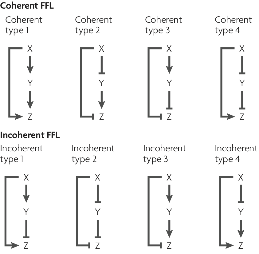
The figure also indicates common abbreviations for these circuits: e.g., C2-FFL is the coherent FFL of type 2 and I4-FFL is the incoherent FFL of type 4.

The most-encountered FFLs

While FFLs in general are motifs, some FFLs are more often encountered than others. In the figure below, also taken from Alon (Nature Rev. Genet., 2007), we see relative abundance of the eight different FFLs in E. coli and S. cerevisiae. Two FFLs, C1-FFL and I1-FFL stand out as having much higher abundance than the other six.

We will take a look at these two FFLs in turn to see what features they might provide. First, though, we need to consider the logic of regulation by more than one transcription factor.

Logic of regulation at Z

Because X and Y both regulate Z in an FFL, we need to specify how they do that. For the sake of illustration, let us assume we are discussing C1-FFL, where

$$ Y \rightarrow Z\\ X \rightarrow Z $$

We distinguish between two semantics:

• One can imagine a scenario where both X and Y need to be present to turn on Z. For example, they could be binding partners that together serve to recruit polymerase to the promoter. To get expression of Z, we must have X AND Y.

• Conversely, if either X or Y may each alone activate Z, we have that Z is expressed if X OR Y.

So, to fully specify an FFL, we need to also specify the logic of how Z is regulated.

An other example is the case where

$$ Y -\mid Z\\ X -\mid Z $$

and the composition is via an AND resulting in (NOT X) AND (NOT Y) = NOR(X,Y); a gate that we know from before.

Completing the example FFL with, say: $$ X \rightarrow Y -\mid Z\\ X -\mid Z $$

results in a behavior that is related to the digital circuit:

with schemdraw.Drawing() as d:
    d.config(unit=0.5)

    # Input X
    X = logic.Line().at((0, 0)).label('X', 'left')

    # Buffer for Y
    BUF = logic.Buf().right().at((2*d.unit, 0)).anchor('in1').label('BUF', 'bottom')
    logic.Line().at(X.end).to(BUF.in1)

    # NOR gate for Z
    NOR = logic.Nor().right().at((6*d.unit, 0)).anchor('in1').label('NOR', 'bottom')

    # Connect buffer output to NOR input 1 (Y)
    logic.Line().at(BUF.out).to(NOR.in1)
    logic.Line().left().at(NOR.in1).label('Y', 'top')

    # Connect X directly to NOR input 2 with "L-shaped" wire
    X_down = logic.Line().down(2*d.unit).at(X.end).idot()
    X_horiz = logic.Line().right(NOR.in2.x - X_down.end.x).at(X_down.end)
    logic.Line().at(X_horiz.end).to(NOR.in2).label('X', 'top')

    # Label NOR output
    logic.Line().right().at(NOR.out).label('Z', 'right')

Logic with two activators

First, let us fix the quantities of our model:

• We choose $C, Y, Z$ to be concentrations as opposed to rates like in the NOR before.
• We use $f(x,y)$ to model a normalized (dimensionless and within $[0,1]$) expression rate of $Z$.

Call $f_{AND}(x,y)$ the normalized expression rate of Z = X AND Y. Likewise, $f_{OR}(x,y)$ denotes the normalized expression rate of Z = X OR Y.

Let $f$ be either $f_{AND}$ or $f_{OR}$. Using a simple 1st-order dynamic model as an approach, the concentration of $Z$ follows:

\begin{align} \frac{\mathrm{d}z}{\mathrm{d}t} = \beta_0\,f(x, y) - \gamma z\enspace, \end{align}

where $\beta_0$ is the maximal production rate and $\gamma$ is its degradation/dilution rate.

Our goal is to specify the dimensionless function $f(x, y)$ that encodes the appropriate logical functions.

The function depends on the underlying mechanistics. In all cases, however, there are basic constraints that we expect to hold. For example, for AND, we would like limits $x,y \to \infty$ (i.e., both inputs logically 1) result in $1$ and $x = 0$ or $y = 0$ (one of the inputs being logically 0) result in $0$. One readily verifies that this is the case.

There is a method from statistical physics to systematically derive such formulas. Essentially we are interested in the formula \begin{align} f = \frac{\sum \text{active promoter probabilities}}{\sum \text{all promoter probabilities}} \end{align} Instead of probabilities, we can also use values that are proportional to probabilities with the same proportionality factor $C$ (statistical weight). Factor $C$ then simply cancels in the fraction. Denote the state concentrations by:

• Unbound promoter: $[P]$
• Bound by X: $[PX]$
• Bound by Y: $[PY]$
• Bound by X and Y: $[PXY]$

Let us assume independent binding of the repressors $X$ and $Y$ to their binding sites, and zero or excessive amounts of both repressor like in the Hill approximation. We choose to write probabilities relative to $C = [P]$.

State	Reaction	Equilibrium Relation	Statistical Weight (relative to $[P]$)	Notes
Unbound	—	—	1	Reference state (baseline energy = 0)
X bound	$X + P \leftrightarrow PX$	$K_x = \frac{[X][P]}{[PX]}$	$\frac{[PX]}{[P]} = \frac{[X]}{K_x}$	Independent binding of X
Y bound	$Y + P \leftrightarrow PY$	$K_y = \frac{[Y][P]}{[PY]}$	$\frac{[PY]}{[P]} = \frac{[Y]}{K_y}$	Independent binding of Y
Both bound (sequential)	$Y + PX \leftrightarrow PXY$	$K_y =\frac{[Y][PX]}{[PXY]}$	$\frac{[PXY]}{[P]} = \frac{[X][Y]}{K_x K_y}$	Independent binding of Y
	$X + PY \leftrightarrow PXY$	$K_x = \frac{[X][PY]}{[PXY]}$	$\frac{[PXY]}{[P]} = \frac{[X][Y]}{K_x K_y}$	Independent binding of X

For example, for an AND we assume that only the state where both binding sites of the promoter are bound is active. The statistical weight of the active states is \begin{align} \left(\frac{x}{K_x}\right)^{n_x} \cdot \left(\frac{y}{K_y}\right)^{n_y} \end{align} For the statistical weight of all states (both sites unbound, X site bound, Y site bound, both X and Y sites bound) we have \begin{align} 1 + \left(\frac{x}{K_x}\right)^{n_x} + \left(\frac{y}{K_y}\right)^{n_y} + \left(\frac{x}{K_x}\right)^{n_x} \cdot \left(\frac{y}{K_y}\right)^{n_y} = \left(1 + \left(\frac{x}{K_x}\right)^{n_x}\right) \left(1 + \left(\frac{y}{K_y}\right)^{n_y}\right) \end{align} The same can the done for OR assuming that all except the unbound state are active.

We thus obtain: \begin{align} f_{AND}(x,y) &= \frac{(x/K_x)^{n_x} (y/K_y)^{n_y}}{\left(1 + \left(\frac{x}{K_x}\right)^{n_x}\right) \left(1 + \left(\frac{y}{K_y}\right)^{n_y}\right)}\\[2em] f_{OR}(x,y) &= \frac{(x/K_x)^{n_x} + (y/K_y)^{n_y} + (x/K_x)^{n_x} (y/K_y)^{n_y}}{\left(1 + \left(\frac{x}{K_x}\right)^{n_x}\right) \left(1 + \left(\frac{y}{K_y}\right)^{n_y}\right)} \end{align}

In what follows, we will substitute $x/K_x \to x$ and $y/K_y \to y$. This is just for simplicity. Note that now, $x$ and $y$ are dimensionless.

\begin{align} f_{AND}(x,y) &= \frac{x^{n_x} y^{n_y}}{(1 + x^{n_x})(1 + y^{n_y})}\\[1em] f_{OR}(x,y) &= \frac{x^{n_x} + y^{n_y} + x^{n_x} y^{n_y}}{(1 + x^{n_x})(1 + y^{n_y})} \end{align}

We can make plots of these functions to demonstrate how they represent the respective logic.

# Get x and y values for plotting
x = np.linspace(0, 3, 200)
y = np.linspace(0, 3, 200)
xx, yy = np.meshgrid(x, y)

# Parameters (Hill functions)
# increase them to make it more digital
nx: float = 3.0  # 20.0
ny: float = 3.0  # 20.0

# Regulation functions
def aa_and(x: np.ndarray, y: np.ndarray, nx: float, ny: float):
    comb = x ** nx * y ** ny
    return  comb / ((1 + x ** nx)*(1 + y ** ny))


def aa_or(x: np.ndarray, y: np.ndarray, nx: float, ny: float):
    comb = x ** nx + y ** ny + x ** nx * y ** ny
    return comb / ((1 + x ** nx)*(1 + y ** ny))

# plot it
contour_fun(xx, yy,
            aa_and(xx, yy, nx, ny),
            title="two activators, AND logic")

contour_fun(xx, yy,
            aa_or(xx, yy, nx, ny),
            title="two activators, OR logic")

Same with two repressors or one repressor and one activator

We can do the same with two repressors instead of two activators. The AND case where X and Y are both repressors is (NOT X) AND (NOT Y) = NOR(X,Y). Here, either repressor (or both) can shut down gene expression.

For the OR of two repressors, we have (NOT X) OR (NOT Y) = NAND(X,Y).

Functions can again be obtained by the statistical weight method: \begin{align} f_{NOR}(x,y) &= \frac{1}{(1 + x^{n_x}) (1 + y^{n_y})}\\[1em] f_{NAND}(x,y) &= \frac{1 + x^{n_x} + y^{n_y}}{(1 + x^{n_x}) ( 1 + y^{n_y})} \end{align}

Side note: The $f_{NOR}(x,y)$ function is different from the one we used to model the NOR. This has some reasons:

• Here, we use a model that maps concentrations to rates.

• This function is mechanistically motivated from a repressor that blocks if it is bound to either of the promoter sites. This results in the two repression Monod terms being multiplied.

  In the NOR gate with Tandem Promoters, we had only the right promoter blocking the left one but not the left one blocking the right one. In the split gate, we even added both activities without any of the promoter blocking the other one.

When modeling, we thus have to be careful what the underlying mechanism is.

The same method can be applied to cases of one repressor and one activator. Calling the activator $A$ and the repressor $R$, AND logic means A AND (NOT R), and OR logic means A OR (NOT R).

\begin{align} f_{ANDNOT}(x,y) &= \frac{x^{n_x}}{(1 + x^{n_x})(1 + y^{n_y})}\\[1em] f_{ORNOT}(x,y) &= \frac{1 + x^{n_x} + x^{n_x}y^{n_y}}{(1 + x^{n_x})(1 + y^{n_y})} \end{align}

with the following plot

# Regulation functions
def ar_and(x, y, nx, ny):
    return x ** nx / ((1 + x ** nx)*(1 + y ** ny))


def ar_or(x, y, nx, ny):
    return (1 + x ** nx + x ** nx * y ** ny) / ((1 + x ** nx)*(1 + y ** ny))

# Parameters (Hill functions)
# increase them to make it more digital
nx = 3  # 20
ny = 3  # 20

# Generate plots
contour_fun(xx, yy,
            ar_and(xx, yy, nx, ny),
            title="ANDNOT: X activates, Y represses, with AND logic")

contour_fun(xx, yy,
            ar_or(xx, yy, nx, ny),
            title="ORNOT: X activates, Y represses, with OR logic")

Numerical solution of the FFL circuits

To specify the dynamical equations so that we may numerically solve them, we need to specify the functions $f_y$ and $f_z$ along with their Hill coefficients. The function $f_y$ is either an activating or repressive Hill function, and the functions $f_z$ have already been defined as aa_and(), aa_or(), etc., above.

Let's proceed to code up the right-hand side of the dynamical equations for FFLs. It is convenient to define a function that will give back a function that we can use as the right-hand side we need to specify to scipy.integrate.odeint(). Remember that odeint() requires a function of the form func(yz, t, *args), where yz is an array containing the values of $y$ and $z$. For convenience, our function will return a function with call signature rhs(yz, t, x), where x is the value of $x$ at a given time point.

from typing import Literal

# Regulation functions
def a_hill(x, nx):
    comb = x ** nx
    return  comb / (1 + comb)


def r_hill(x, nx):
    comb = x ** nx
    return 1 / (1 + comb)


# get FFL functions
def ffl_rhs(beta, gamma, kappa, n_xy, n_xz, n_yz, ffl: str, logic: Literal["and", "or"]):
    """Return a function with call signature fun(yz, t, input_x_fun) that computes
    the right-hand side of the dynamical system for an FFL. Here,
    `yz` is a length two array containing concentrations of Y and Z.
    """
    if ffl[:2].lower() in ("c1", "c3", "i1", "i3"):
        fy = lambda x: a_hill(x, n_xy)
    else:
        fy = lambda x: r_hill(x, n_xy)

    if ffl[:2].lower() in ("c1", "i4"):
        if logic.lower() == "and":
            fz = lambda x, y: aa_and(x, y, n_xz, n_yz)
        else:
            fz = lambda x, y: aa_or(x, y, n_xz, n_yz)
    elif ffl[:2].lower() in ("c4", "i1"):
        if logic.lower() == "and":
            fz = lambda x, y: ar_and(x, y, n_xz, n_yz)
        else:
            fz = lambda x, y: ar_or(x, y, n_xz, n_yz)
    elif ffl[:2].lower() in ("c2", "i3"):
        if logic.lower() == "and":
            fz = lambda x, y: ar_and(y, x, n_yz, n_xz)
        else:
            fz = lambda x, y: ar_or(y, x, n_yz, n_xz)
    else:
        if logic.lower() == "and":
            fz = lambda x, y: rr_and(x, y, n_xz, n_yz)
        else:
            fz = lambda x, y: rr_or(x, y, n_xz, n_yz)

    def rhs(yz, t, input_x_fun):
        """System as d/dt"""
        x = input_x_fun(t)
        y, z = yz
        dy_dt = beta * fy(kappa * x) - y
        dz_dt = gamma * (fz(x, y) - z)
        return np.array([dy_dt, dz_dt])

    return rhs

To study the dynamics, we will investigate how the circuit responds to a step up in concentration of X, assuming all concentrations are initially zero, and how a circuit at steady state with nonzero concentration of X responds to a step down in X to zero.

def solve_ffl(
    beta, gamma, kappa, n_xy, n_xz, n_yz, ffl: str, logic: Literal["and", "or"], t: np.ndarray, t_step_down: float, x_0: float
):
    """Solve an FFL. The dynamics are given by
    `rhs`, the output of `ffl_rhs()`.
    """
    if t[0] != 0:
        raise RuntimeError("time must start at zero.")

    rhs = ffl_rhs(beta, gamma, kappa, n_xy, n_xz, n_yz, ffl, logic)

    # define a down-step input
    def input_x_fun(t) -> float:
        if t < t_step_down:
            return x_0
        else:
            return 0.0

    # Integrate
    return scipy.integrate.odeint(rhs, np.zeros(2), t, args=(input_x_fun,))

Finally, we can write a function to solve and plot the dynamics of an FFL for a unit step.
At the end of this notebook, we have a dashboard to explore the C1-FFL and I1-FFL, but for the pedagogical purposes of exposing design principles here, we will vary the parameters one-by-one as we work down the notebook.

colors = ['red', 'green', 'blue']

def plot_ffl(
    beta=1.0,
    gamma=1.0,
    kappa=1.0,
    n_xy=1.0,
    n_xz=1.0,
    n_yz=1.0,
    ffl="c1",
    logic="and",
    t=np.linspace(0, 20, 200),
    t_step_down=10.0,
    x_0=1.0,
    normalized=False,
):
    yz = solve_ffl(
        beta, gamma, kappa, n_xy, n_xz, n_yz, ffl, logic, t, t_step_down, x_0
    )
    y, z = yz.transpose()

    # Generate x-values
    if t[-1] > t_step_down:
        t_x = np.array(
            [-t_step_down / 10, 0, 0, t_step_down, t_step_down, t[-1]]
        )
        x = np.array([0, 0, x_0, x_0, 0, 0])
    else:
        t_x = np.array([-t[-1] / 10, 0, 0, t[-1]])
        x = np.array([0, 0, x_0, x_0])

    # Add left part of y and z-values
    t = np.concatenate(((t_x[0],), t))
    y = np.concatenate(((0,), y))
    z = np.concatenate(((0,), z))

    # Set up figure
    plt.figure()
    plt.xlabel("dimensionless time")
    plt.ylabel(f"{'norm. ' if normalized else ''}dimensionless conc.")

    if normalized:
        x = x / x.max()
        y = y / y.max()
        z = z / z.max()
    
    plt.plot(t_x, x, color=colors[0], label="x")
    plt.plot(t, y, color=colors[1], label="y")
    plt.plot(t, z, color=colors[2], label="z")
    plt.legend()

C1-FFL with AND: Sign-sensitive delay

Now that we have laid the computational groundwork, we will proceed to an analysis of the first of the two over-represented FFLs, the C1-FFL.

with schemdraw.Drawing() as d:
    d.config(unit=0.5)

    # Input X
    X = logic.Line().at((0, 0)).label('X', 'left')

    # Buffer for Y
    BUF = logic.Buf().right().at((2*d.unit, 0)).anchor('in1')
    logic.Line().at(X.end).to(BUF.in1)

    # NOR gate for Z
    AND = logic.And().right().at((6*d.unit, 0)).anchor('in1')

    # Connect buffer output to AND input 1 (Y)
    logic.Line().at(BUF.out).to(AND.in1)
    logic.Line().left().at(AND.in1).label('Y', 'top')

    # Connect X directly to AND input 2 with "L-shaped" wire
    X_down = logic.Line().down(2*d.unit).at(X.end).idot()
    X_horiz = logic.Line().right(AND.in2.x - X_down.end.x).at(X_down.end)
    logic.Line().at(X_horiz.end).to(AND.in2).label('X', 'top')

    # Label AND output
    logic.Line().right().at(AND.out).label('Z', 'right')

Let's look at the dynamics for a sudden step up and step down in X.

# Parameter values
beta = 5
gamma = 1
kappa = 1
n_xy, n_yz = 3, 3
n_xz = 5

# Plot
plot_ffl(beta, gamma, kappa, n_xy, n_xz, n_yz, ffl="c1", logic="and")

Notice that there is a time delay for production of $Z$ upon stimulation with $X$. This is a result of the AND logic. Though $X$ has immediately come up, we have to wait for the signal to pass through $Y$ for $Z$ to come up. This off-response is perhaps more apparent if we normalize the signals.

plot_ffl(
        beta,
        gamma,
        kappa,
        n_xy,
        n_xz,
        n_yz,
        ffl="c1",
        logic="and",
        normalized=True,
)

Here, the delay is more apparent, as is the fact that both Y and Z have their levels immediately decrease when the X stimulus is removed. So, we have arrived at a design principle: The C1-FFL with AND logic has an on-delay, but no off-delay.

The magnitude of the delay can be tuned

How might we get a longer delay? If we decrease $\kappa = k_{xz}/k_{yz}$, we are increasing the disparity between the threshold levels needed to turn on gene expression. This should result in a longer time delay. Let's try it!

# Update parameter
kappa = 0.001

plot_ffl(
        beta,
        gamma,
        kappa,
        n_xy,
        n_xz,
        n_yz,
        ffl="c1",
        logic="and",
        normalized=True
)

Making a sweep

Indeed, the delay is longer with small $\kappa$. We can quantify how the delay changes with $\kappa$ by plotting how long it takes for the $z$ level to rise to ten percent of its steady state value for various values of $\kappa$.

THRESHOLD_FRACTION = 0.1  # 10% of steady state

tau = []
kappa_vals = np.logspace(-1, 2, 200)

# Finer time points
t_ = np.linspace(0, 20, 5000)

for kappa in kappa_vals:
    yz = solve_ffl(
        beta, gamma, kappa, n_xy, n_xz, n_yz, "c1", "and", t_, np.inf, 1
    )
    z_thresh = yz[-1, 1] * THRESHOLD_FRACTION
    i = np.nonzero(yz[:, 1] > z_thresh)[0][0]
    tau.append(t_[i])
    
plt.figure()
plt.plot(kappa_vals, tau)
plt.xlabel(r'$\kappa$')
plt.ylabel(f'rise time to {THRESHOLD_FRACTION*100}%')
plt.xlim([0,5])

(0.0, 5.0)

The delay does not change substantially, only about a factor of three over many orders of magnitude.

Short Pulse Filter

Now, let's see what happens if we have a shorter pulse. Due to its similarly with the cascade we previously studied, the delay feature of the C1-FFl should also filter our short pulses.

# Shorter pulse
t = np.linspace(0, 1, 200)
t_step_down = 0.1

# Reset kappa and ultrasensitivity
kappa = 1
n_xy, n_xz, n_yz = 3, 5, 3

plot_ffl(
        beta,
        gamma,
        kappa,
        n_xy,
        n_xz,
        n_yz,
        ffl="c1",
        logic="and",
        t=t,
        t_step_down=t_step_down,
        normalized=False,
)

The shorter pulse is ignored in the Z-response because of the delay.

The sign-sensitivity of the delay is reversed with OR logic

We will now investigate the response of the circuit to the same stimulus, except with OR logic.

plot_ffl(
        beta,
        gamma,
        kappa,
        n_xy,
        n_xz,
        n_yz,
        ffl="c1",
        logic="or",
        normalized=False,
)

Again, let's normalize to see it more clearly:

plot_ffl(
        beta,
        gamma,
        kappa,
        n_xy,
        n_xz,
        n_yz,
        ffl="c1",
        logic="or",
        normalized=True,
)

Sign sensitive delay is observed experimentally

The arabinose and lac systems in E. coli are both turned on by cyclic AMP (cAMP), which stimulates production of CRP, but they have different architectures, shown below.

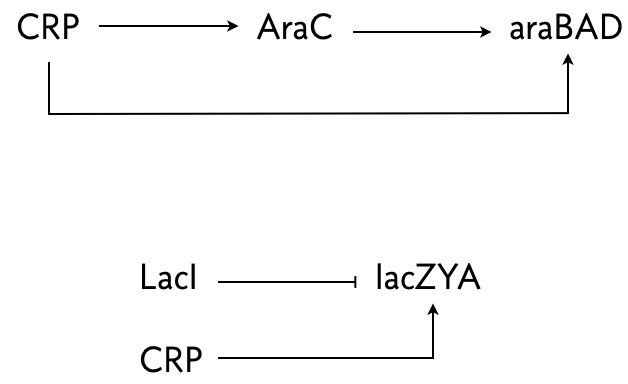
In both system where multiple species regulate one, AND logic is employed.

Mangan, Zaslaver, and Alon (J. Molec. Biol., 2003) performed an experiment where they put a fluorescent reporter under control of the products of these two systems, araBAD and lacZYA, respectively. In the lac system, IPTG was also present, so LacI was inhibited. Thus, lacZYA production was directly activated by CRP. Conversely, the arabinose system is a C1-FFL.

They measured the fluorescent intensity in cells that were suddenly exposed to cAMP. The response of these two systems to the sudden jump in cAMP is shown in the left plot below.

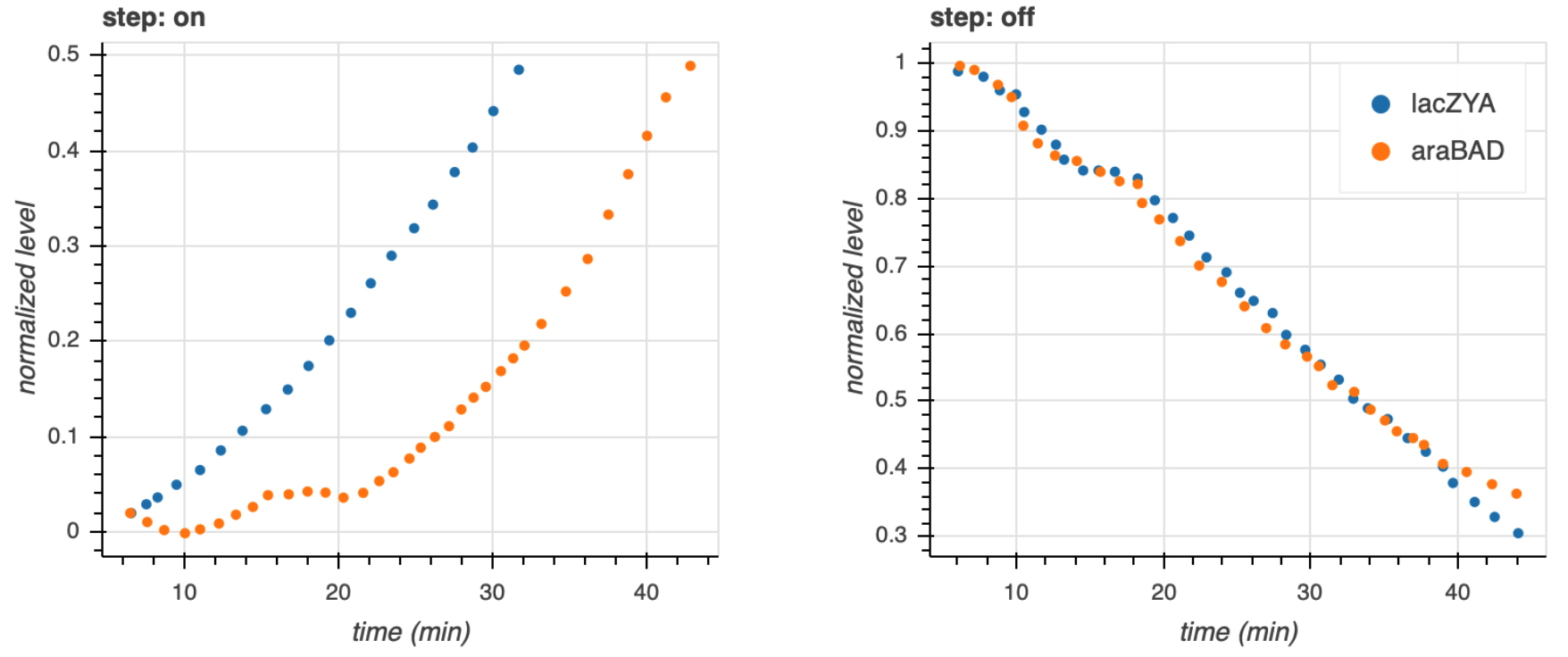
While the lac system response immediately, the arabinose system exhibits a lag before responding. This is indicative of a time delay for a step on in the stimulus for a C1-FFL. Conversely, after these systems come to steady state and are subjected to a sudden decrease in cAMP, both the arabinose and lac systems respond immediately, without delay, which is also expected from a C1-FFL with AND logic.

Kalir, Mangan, and Alon (Mol. Sys. Biol., 2005) did a similar experiment with another C1-FFL circuit found in E. coli, this time with OR logic. A circuit that regulates flagella formation is a "decorated" C1-FFL, shown below. We say it is decorated because the "Y" gene, in this case FliA, is also autoregulated. Importantly, the regulation of FliL by FliA and FlhDC is governed by OR logic.

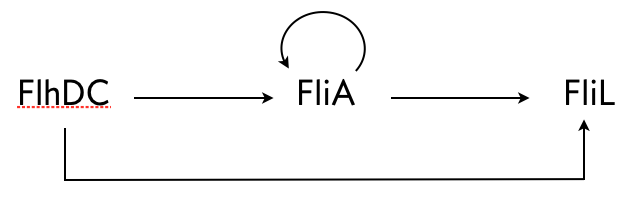
They used engineered cells in which the FlhDC gene was under control of a promoter which could be induced with L-arabinose, a chemical inducer. The gene product FliL was altered to be fused to GFP to enable fluorescent monitoring of expression levels. To consider a circuit where FlhDC directly activates FliL, the authors used mutant E. coli cells in which the fliA gene was deleted.

Because of the OR logic, we would expect that a sudden increase in FlhDC would result in both the wild type and mutant cells to respond at the same time, that is with no delay. Fluorescence traces from these experiments are shown in the left plot, below.

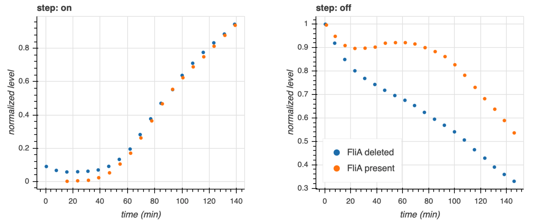
Both strains show a delay, which is due to waiting for FlhDC to be activated, but both come on at the same time. Conversely, after the inducer is removed and FlhDC levels go down, the system with the wild type C1-FFL circuit shows a delay before the FliL levels drop off, while the mutant does not. This demonstrates the sign-sensitivity with OR logic.

I1-FFL with AND: Pulse Generator

We now turn our attention to the other over-represented circuit, the I1-FFL. X activates Y and Z, but Y represses Z. We can use the expressions for production rate under AND and OR logic for one activator/one repressor that we showed above in writing down our dynamical equations. Here, we will consider AND logic.

with schemdraw.Drawing() as d:
    d.config(unit=0.5)

    # Input X
    X = logic.Line().at((0, 0)).label('X', 'left')

    # Buffer for Y
    BUF = logic.Buf().right().at((2*d.unit, 0)).anchor('in1')
    logic.Line().at(X.end).to(BUF.in1)

    # NOR gate for Z
    AND = logic.And(inputnots=[1]).right().at((6*d.unit, 0)).anchor('in1')

    # Connect buffer output to AND input 1 (Y)
    logic.Line().at(BUF.out).to(AND.in1)
    logic.Line().left().at(AND.in1).label('Y', 'top')

    # Connect X directly to AND input 2 with "L-shaped" wire
    X_down = logic.Line().down(2*d.unit).at(X.end).idot()
    X_horiz = logic.Line().right(AND.in2.x - X_down.end.x).at(X_down.end)
    logic.Line().at(X_horiz.end).to(AND.in2).label('X', 'top')

    # Label AND output
    logic.Line().right().at(AND.out).label('Z', 'right')

For this circuit, we will investigate the response in Z to a sudden, sustained step in stimulus X. We will choose $\gamma = 10$, which means that the dynamics of Z are faster than Y.

# Parameter values
beta = 5
gamma = 10
kappa = 1
n_xy, n_yz = 3, 3
n_xz = 5
t = np.linspace(0, 10, 200)

# Set up and solve
plot_ffl(
        beta,
        gamma,
        kappa,
        n_xy,
        n_xz,
        n_yz,
        ffl="i1",
        logic="and",
        t=t,
        t_step_down=np.inf,
        normalized=False,
)

We see that Z pulses up and then falls down to its steady state value. This is because the presence X leads to production of Z due to its activation. X also leads to the increase in Y, and once enough Y is present, it can start to repress Z. This brings the Z level back down toward a new steady state where the production rate of Z is a balance between activation by X and repression by Y. Thus, the I1-FFL with AND logic is a pulse generator.

---

License & Attribution: This page is adapted from material by Michael Elowitz and Justin Bois (© 2021–2025), licensed under CC BY-NC-SA 4.0.